Building a self-balancing robot is one of those things that every hobbyist and engineer want to do. But there are a few hurdles for a lot of people. There is the theory on the one hand and then there is the mechanics on the other. In this and the next few posts, I will show you a self-balancing robot I recently built and will explain in details on some of the most important aspects.
Before I started building, I laid down a couple of my own requirements:
- Low cost
- Relatively simple controls
I thought that the low cost requirement is an important one as people tend to shy away from projects that need hundreds of dollars. Luckily, you can build a surprisingly good balancing robot without having to spend a fortune, especially if you are willing to build all the electronics yourself.
Here is the bill of material in my build:
Platform: Toy truck (0 – $20)
Controller: ATmega328P (~$4)
Accelerometer: MMA8453Q (~$2)
Gyroscope: LPY450AL ($4)
H-Bridge: SN754410 (~$2)
Miscellaneous: ~$10
If you have a toy truck lying around, you can then re-purpose it without having to buy one (I re-cycled a broken one from my son), this would cut your total cost down to around $20.
Simplicity is another important factor. In order for the control algorithm to work successfully, you have to understand the principle behind it. The more complex the control algorithm is the more there is room for error and thus keeping everything simple is the key to a successful build. It is a good idea to keep things simple and only move on to more complex implementations after you have understood everything.
Now let’s move on to to the theory. I am not going to bore you with the excessive math here but if you are interested, there are a lot of excellent sources for the math behind this. For those who already know the theory and just want to see the implementation, you will have to wait for my next post.
The General Idea
Making a self-balancing robot is essentially solving the classic inverted pendulum problem. While the math is a bit complex, the essence is quite simple: the goal of the control loop is to adjust the wheels’ position so that the inclination angle remains stable at a pre-determined value (e.g. the angle when the robot is balanced). When the robot starts to fall in one direction, the wheels should move in the falling direction to correct the inclination angle. And heuristics tell us that when the deviation from equilibrium is small, we should move “gently” and when the deviation is large we should move more quickly.
To simplify things a little bit, I limited the robot’s movement to be on a straight line (e.g. only forward and backward motion but no turning) and thus both wheels are moved at the same speed in the same direction. Under this restriction the calculations become much simpler as we only need to worry about sensor readings on a single plane. If you need to allow the robot to make turns, then you will have to control each wheel independently. The general principle remains the same nevertheless since the falling direction of the robot is still restricted to a single plane.
In the next couple of sections, we will discuss the method used to accurately estimate the inclination angle.
Estimating the Inclination Angle with an Accelerometer
As mentioned above, we would need to get a good measurement of the current inclination angle in order to control the robot’s movements. Let’s first examine how to use an accelerometer alone to measure the inclination angle.
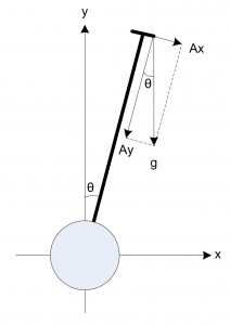
Suppose that the robot is a stationary position illustrated below (viewed from the side, accelerometer is placed on the top of the robot, perpendicular to the body):

The inclination angle can be calculated as:
\[\theta=tan^{-1}\frac{A_x}{A_y}=sin^{-1}\frac{A_x}{\sqrt{A_x^2 + A_y^2}}=sin^{-1}\frac{A_x}{g}\]
In the equations above, Ax is the accelerometer reading along its x axis and Ay is the accelerometer reading on its y axis. When the robot is stationary, g is the gravitational constant (which translates into the accelerometer reading on the y axis when the accelerometer is lying flat). In this inverted pendulum application, we are only interested in calculations where the inclination angle is small since our goal is to ensure that the deviation from equilibrium (typically equilibrium is reached when the inclination angle is close to 0 depending on the weight distribution of the robot) is as small as possible. So we can further simply the above equation for small inclination angles:
\[\theta\approx sin(\theta)=\frac{A_x}{g} \quad \text{… (1)}\]
By only measuring the x axis reading of the accelerometer we can get a rough estimate of the inclination angle. Of course, this is under the assumption that the robot is standing still. In reality, when the robot is not in balance it will accelerate towards the direction it is falling and thus the x axis reading of the accelerometer will be slight more than Ax due to the acceleration. At the same time, the y axis reading will be slightly less than the reading in standstill condition (Ay). As a result, the combined vector will deviate from g. But when the accelerometer is placed near the center of gravity of the robot, the acceleration along the x axis is small in near-equilibrium conditions. So the above equation will exhibit some small error, but it remains a good approximation of the inclination angle.
Accelerometer tends to be very sensitive to the accelerations introduced due to movement or vibration and thus the sensor readings will contain some level of noise, which can not be removed easily. So by relying on accelerometer readings alone, we can not get a reliable inclination angle estimate. To address this issue, we will have to rely on some other measurements.
Estimating the Inclination Angle with a Gyroscope
Gyroscope can measure the rate at which the rotation is taking place. And the rotation angle for a given time interval is governed by:
\[\theta(t)=\int_{t_1}^{t_2}G(t)dt\]
Where G(t) is the gyroscope reading with respect to the rotation direction. When the time interval is small enough, the gyroscope reading can be treated as a constant and thus the above equation can be approximated as:
\[\theta(t) \approx \theta(t_1) + G(t)(t_2 – t_1) = \theta(t_1) + G(t)\Delta t \quad \text{… (2)}\]
Unlike the accelerometer, gyroscope measurement is largely immune to none angular movement and thus far less susceptible to vibrations and lateral accelerations mentioned previously. But since the angular measurement is cumulative, any minute error in measurements will manifest over time which causes the estimated angle to deviate from the true value. This is the so called drifting effect. Thus gyroscope alone cannot be used to reliably measure the inclination angle either.
Sensor Fusion
To address the issue of measurement noises and the limitations of measurements by either the accelerometer or gyroscope alone, we will need to combine the readings from both the accelerometer and the gyroscope in a meaningful way so that we could use the strengths from both sensors to obtain a more accurate result than either measurement alone could provide. This is the classic application of sensor fusion. Since accelerometers can provide accurate angle calculations when there is no acceleration and gyroscope can provide accurate short-time angle measurements. These complementary traits are ideal candidates for sensor fusion.
Some sources confuse the concept of sensor fusion with data filtering. As mentioned before, the concept of sensor fusion is to combine the measurements from multiple sensors in hope to obtain better measurement results. This can be done either in conjunction to or independent of filtering.
Like many processes in the physical world, sensor readings from the accelerometer and the gyroscope can be modeled as the true measurements with added white Gaussian noise (AWGN). Many filters in the least mean square filters family are suitable for this kind of stochastic process.
Kalman filter is one such adaptive filters that can be used to filter the sensor data from accelerometer and gyroscope. Even though the implementation of Kalman filter is quite straight forward, in order for the filter to be optimal we needed to know the precise underlying model of the system and we also need to be able to reliably estimate the noise covariance matrices. Without any reliable information on these parameters, the filter may still work but will not be in an optimal sense. Simpler methods can be used in situations where the these parameters are unknown and can still achieve reasonably good result.
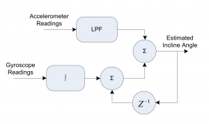
So, to keep the implementation simple, I used the method illustrated below where the estimated value is a linear combination of the filtered measurements from both the accelerometer and the gyroscope. Each sensor reading is multiplied by a fixed gain:

From the diagram above, you can see that in order to make the accelerometer readings more reliable, the readings are passed through a low pass filter (e.g. averaging over time) to smooth out any sudden change in values. And the gyroscope readings are integrated and then added to the previous estimate to give the current inclination angle reading. Each of the component is weighted and then added together to give the final estimate. Mathematically, the estimated angle can be expressed as follows:
\[\left\{
\begin{array}{l l}\theta_{est}\mid_{t_2}=\alpha(\theta_{est}\mid_{t_1} + G\Delta t) + \beta \theta_{A_x} & \quad\text{… (3)} \\
\alpha+\beta=1 & \quad\text{… (4)} \\
\end{array} \right.
\]
Where G is the gyroscope reading and angle Ax is the angle calculated from the accelerometer reading in equation (1) above.
The weights are chosen such that the gyroscope drift can be corrected reasonably fast while the transient errors in accelerometer measurements do not cause the estimates to vary too much from iteration to iteration. These parameters are sensitive to the sampling period but as a rule of thumb, gyroscope readings should be given a much higher weight (e.g. >0.9) since they are less noise-prone and accelerometer readings should be given a lower weight (e.g. <0.1) as its angle measurement is noisy and it is used only to correct gyroscope's drift. More detailed background information can be found in this excellent presentation. The technique of filtering using linear combination of values from multiple sensors is sometimes casually refereed to as complementary filtering, and it is widely used in many data fusion applications.
It can be shown that this simple filtering technique we used above is after all a special case of the more generic Kalman filter. The main difference is that in our implementation the gain is fixed instead of iteratively computed.
Since we assumed that the noise covariance matrix is unknown (or we chose not to measure it), the complementary filter solution should function as well as a Kalman filter with randomly tuned parameter values if not better. But if the covariance matrix were precomputed according to the underlying physical process model, the Kalman filter would have been the optimal choice.
In my next post, we will use equations (1) to (4) in our implementation.
The Control Loop
In the section above, we discussed the method for obtaining a more accurate inclination angle estimate based on the values provided by both the accelerometer and gyroscope. We now need to control the motor accordingly use this estimate so that the robot can remain stand balanced.
The simplest method one may attempt to employee is to rotate the wheels in the falling direction until the inclination angle reaches the value at which the robot is in balance. Heuristically, the wheel rotation speed should be proportional to the inclination angle (e.g. move faster when the angle is larger and move slower when the angle is smaller) so that the robot moves smoothly. This technique is effectively the simplest PID control with both the I and the D terms set to zero.
In practice though, a full PID implementation is generally needed to make the inverted pendulum stable. This application note from Microchip offers detailed explanations on how to design a PID controller for inverted pendulum application.

