A few days ago, I ran across this article by Dmitri Nesteruk. In his article, he compared the performance between C# and C++ in matrix multiplication. From the data he provided, matrix multiplication using C# is two to three times slower than using C++ in comparable situations.
Even though a lot of optimizations have been done in the .Net runtime to make it more efficient, it is apparent that scientific programming still favors C and C++ because that the performance advantage is huge.
In this article, I will examine some matrix multiplication algorithms that are commonly used and illustrate the efficiencies of the various methods. All the tests are done using C++ only and matrices size ranging from 500×500 to 2000×2000. When the matrix sizes are small (e.g. <50), you can pretty much use any matrix multiplication algorithms without observing any significant performance differences. This is largely due to the fact that the typical stable matrix multiplication algorithms are O(n^3) and sometimes array operation overheads outweigh the benefit of algorithm efficiencies. But for matrices of larger dimensions, the efficiency of the multiplication algorithm becomes extremely important.
Since Dmitri’s article has already captured pretty detailed data using the standard matrix multiplication algorithm, I will not repeat his findings in this article. What I intended to show was the performance data of uBLAS, OpenMP, cBLAS and MATLAB.
The following sample code are compiled under Ubuntu 8.10 64 bit (kernel 2.6.24.23) on Intel Q9450@3.2GHz.
Standard Matrix Multiplication (Single Threaded)
This is our reference code. Later on, I will only show the critical portion of the code and not repeat the common portion of code that initializes/finalizes the arrays. Similarly, the timing method used is also the same across all the tests and will be omitted later on.
float **A, **B, **C;

A = new float*[matrix_size];
B = new float*[matrix_size];
C = new float*[matrix_size];

for (int i = 0 ; i < matrix_size; i++)
{
    A[i] = new float[matrix_size];
    B[i] = new float[matrix_size];
    C[i] = new float[matrix_size];
}

for (int i=0; i<matrix_size; i++)
{
    for (int j = 0 ; j < matrix_size; j++)
    {
        A[i][j]=rand();
        B[i][j]=rand();
    }
}

timeval t1, t2, t;
gettimeofday(&t1, NULL);

for (int i = 0 ; i < matrix_size; i++)
{
    for (int j = 0;  j < matrix_size; j++)
    {
        C[i][j] = 0;
        for (int k = 0; k < matrix_size; k++)
        {
            C[i][j] += A[i][k] * B[k][j];
        }
    }
}

gettimeofday(&t2, NULL);
timersub(&t2, &t1, &t);

cout << t.tv_sec + t.tv_usec/1000000.0 << " Seconds -- Standard" << endl;

for (int i = 0 ; i < matrix_size; i++)
{
    delete A[i];
    delete B[i];
    delete C[i];
}

delete A;
delete B;
delete C;
OpenMP With Two Dimensional Arrays
Using OpenMP, we are able to multiple threads via the #pragma omp directives. For the simple algorithm we used here, the speed increase is almost proportional to the number of available cores within the system.
...
#pragma omp parallel for shared(a,b,c)
for (long i=0; i<matrix_size; i++)
{
    for (long j = 0; j < matrix_size; j++)
    {
        float sum = 0;
        for (long k = 0; k < matrix_size; k++)
        {
            sum +=a[i][k]*b[k][j];
        }
        c[i][j] = sum;
    }
}
...
OpenMP With One Dimensional Arrays
Cache locality is poor using the simple algorithm I showed above. The performance can be easily improved however by improving the locality of the references. One way to achieve better cache locality is to use one dimensional array instead of two dimensional array and as you will see later, the performance of the following implementation has as much as 50% speed gains over the previous OpenMP implementation using two dimensional arrays.
float *a, *b, *c;

a = new float[matrix_size * matrix_size];
b = new float[matrix_size * matrix_size];
c = new float[matrix_size * matrix_size];

for (long i=0; i<matrix_size * matrix_size; i++)
{
    a[i]=rand();
    b[i] = rand();
    c[i] = 0;
}

#pragma omp parallel for shared(a,b,c)
for (long i=0; i<matrix_size; i++)
{
    for (long j = 0; j < matrix_size; j++)
    {
        long idx = i * matrix_size;
        float sum = 0;
        for (long k = 0; k < matrix_size; k++)
        {
            sum +=a[idx + k]*b[k * matrix_size +j];
        }
        c[idx + j] = sum;
    }
}

delete a;
delete b;
delete c;
Boost Library uBLAS (Single Threaded)
Boost library provides a convenient way to perform matrix multiplication. However, the performance is very poor compared to all other approaches mentioned in this article. The performance of the uBLAS implementation is largely on par with that using C# (see benchmarks towards the end of the article). Intel’s Math Kernal Library (MKL) 10.1 does provide functionality to dynamically convert code using uBLAS syntax into highly efficient code using MKL by the inclusion of header file mkl_boost_ublas_matrix_prod.hpp. I have not tried it myself though, but the performance should be comparible to algorithms using the native MKL BLAS interface.
By default (without using MKL’s uBLAS capability) though, uBLAS is single threaded and due to its poor performance and I would strongly suggest avoid using uBLAS in any high performance scientific applications.
matrix<float> A, B, C;

A.resize(matrix_size,matrix_size);
B.resize(matrix_size,matrix_size);

for (int i = 0; i < matrix_size; ++ i)
{
    for (int j = 0; j < matrix_size; ++ j)
    {
        A(i, j) = rand();
        B(i, j) = rand();
    }
}

C =prod(A, B);
Intel Math Kernel Library (MKL) cBLAS
Intel’s Math Kernel Library (MKL) is highly optimized on Intel’s microprocessor platforms. Given that Intel developed this library for its own processor platforms we can expect significant performance gains. I am still surprised at how fast the code runs using cBLAS though. In fact, it was so fast that I doubted the validity of the result at first. But after checking the results against those obtained by other means, those doubts were putting into rest.
The cBLAS matrix multiplication uses blocked matrix multiplication method which further improves cache locality. And it is more than thirty times faster then the fastest OMP 1D algorithm listed above! Another benefit is that by default it automatically detects the number of CPUs/cores available and uses all available threads. This behavior greatly simplifies the code since threading is handled transparently within the library.
float *A, *B, *C;

A = new float[matrix_size * matrix_size];
B = new float[matrix_size * matrix_size];
C = new float[matrix_size * matrix_size];

for (int i = 0; i < matrix_size * matrix_size; i++)
{
    A[i] = rand();
    B[i] = rand();
    C[i] = 0;
}

cblas_sgemm(CblasRowMajor, CblasNoTrans, CblasNoTrans,
    matrix_size,  matrix_size,  matrix_size, 1.0, A,matrix_size,
    B, matrix_size, 0.0, C, matrix_size);
MATLAB (Single Threaded)
MATLAB is known for its efficient algorithms. In fact it uses BLAS libraries for its own matrix calculation routines. The version of MATLAB I have is a little dated (7.0.1), but nevertheless it would be interesting to see how its performance compares with that of latest MKL’s. MATLAB 7 is single threaded, and given the same matrix size, it runs roughly three times slower than the fastest MKL routine listed above (per core).
    a = rand(i,i);
    b = rand(i,i);
    tic;
    c = a*b;
    t = toc
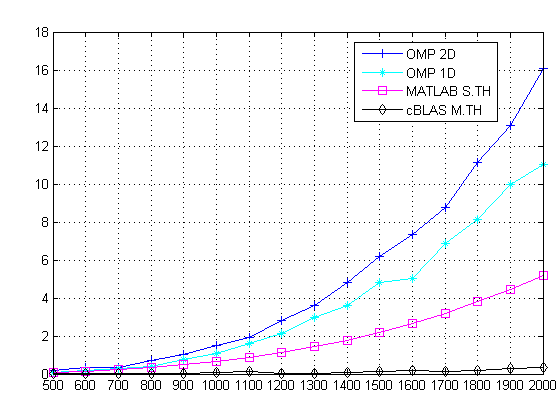
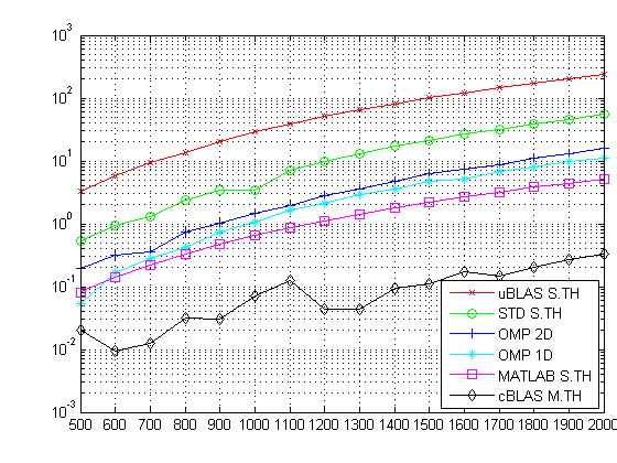
The following table shows the results I obtained by running the code listed above. The results are time in seconds. (note, S.TH means single threaded and M.TH means multi-threaded).
| Size/Algorithm | uBLAS S.TH | STD S.TH | OMP 2D | OMP 1D | MATLAB S.TH | cBLAS M.TH |
| 500×500 | 3.2435 | 0.5253 | 0.1939 | 0.0536 | 0.0810 | 0.0206 |
| 600×600 | 5.7854 | 0.9349 | 0.3223 | 0.1655 | 0.1410 | 0.0093 |
| 700×700 | 9.2292 | 1.2928 | 0.3529 | 0.2797 | 0.2230 | 0.0122 |
| 800×800 | 13.7711 | 2.3746 | 0.7259 | 0.4135 | 0.3320 | 0.0310 |
| 900×900 | 20.3245 | 3.4983 | 1.0146 | 0.7449 | 0.4740 | 0.0306 |
| 1000×1000 | 28.8345 | 3.4983 | 1.4748 | 1.0548 | 0.6530 | 0.0700 |
| 1100×1100 | 38.2545 | 7.0240 | 1.9383 | 1.6257 | 0.8620 | 0.1250 |
| 1200×1200 | 50.4964 | 9.9319 | 2.8411 | 2.1215 | 1.1170 | 0.0440 |
| 1300×1300 | 64.5064 | 12.8344 | 3.6277 | 2.9720 | 1.4250 | 0.0440 |
| 1400×1400 | 81.1826 | 17.1119 | 4.8309 | 3.5977 | 1.7760 | 0.0938 |
| 1500×1500 | 100.1330 | 21.0622 | 6.1689 | 4.8022 | 2.1870 | 0.1111 |
| 1600×1600 | 120.3400 | 26.4316 | 7.3189 | 5.0451 | 2.6490 | 0.1699 |
| 1700×1700 | 145.8550 | 31.2706 | 8.7525 | 6.8915 | 3.1870 | 0.1452 |
| 1800×1800 | 174.6860 | 38.9293 | 11.1060 | 8.1316 | 3.7940 | 0.1989 |
| 1900×1900 | 206.0520 | 45.8589 | 13.0832 | 9.9527 | 4.4450 | 0.2725 |
| 2000×2000 | 240.7820 | 55.4392 | 16.0542 | 11.0314 | 5.1820 | 0.3359 |
The following figure shows the results. Since uBLAS and single threaded matrix multiplications took significantly longer to compute, I did not include them in the figure below.
The following figure shows the same data but uses log-scale Y axis instead so that all the data can show up nicely. You can get a sense of various algorithms’ efficiencies here:


